Software
 Exclusive Software. Developed in C++ with all the usual windows functions (open, close, pan, zoom, print). After years of evolution, resulted in a powerful but user-friendly system, fully configurable for each user requirements. It can handle several test simultaneously with interesting comparison and analysis tools, a practical show/no show command, different curves colors and traces making results comparisons a really easy job.
Different types of graphics, charts & reports are available.
A pass / no pass curve analyzer and a production module are other available functions.
Exclusive Software. Developed in C++ with all the usual windows functions (open, close, pan, zoom, print). After years of evolution, resulted in a powerful but user-friendly system, fully configurable for each user requirements. It can handle several test simultaneously with interesting comparison and analysis tools, a practical show/no show command, different curves colors and traces making results comparisons a really easy job.
Different types of graphics, charts & reports are available.
A pass / no pass curve analyzer and a production module are other available functions.
Shock absorbers | How is a sinusoidal test?
First of all we want to define how occurs a sinusoidal test, whatever its stroke and frequency, occurs as following: Firstly is the expansion cycle. It starts with maximum acceleration from the TDC (top dead center), and zero speed; reaching then the maximum speed point (in the middle of the stroke). This maximum speed is determined by the configured stroke and frequency; at that moment the acceleration is zero. From that point the expansion cycle continues but with a decreasing speed (decelerate period) up to the BDC (bottom dead center), reaching there with zero speed. At that moment, in the BDC point, the compression cycle starts. The compression cycle also has two periods: acceleration from zero speed to Vmax (in the middle of the stroke); and a decelerate cycle period, from Vmax to zero speed, finishing in the TDC.
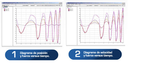
7 kinds of graphics and a newfangled system PASS NO PASS
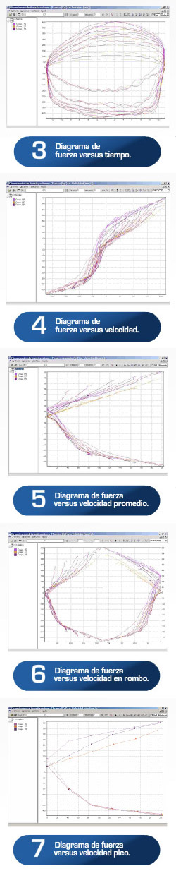 3- The graphic is performed in clockwise, making first the expansion part (the inferior with negative force values) and then the compression one. Knowing this developing form of the graphic, the user can analyze different kinds of failures that a shock may be having.
It is ideal for analyzing the hydraulic behavior of the shock, not for the developing of it.
3- The graphic is performed in clockwise, making first the expansion part (the inferior with negative force values) and then the compression one. Knowing this developing form of the graphic, the user can analyze different kinds of failures that a shock may be having.
It is ideal for analyzing the hydraulic behavior of the shock, not for the developing of it.
4- The graphic is performed in counterclockwise, making: first the expansion part, where we have two speed branches, one the expansion with acceleration branch which is done first and then the expansion with deceleration branch, passing next to the compression cycle, where again passes first for the compression with acceleration branch and finally for the deceleration one. This graphic has many derivations as it can be seen next.
5- It is another way to show the graphic #4. Here the velocity is always positive, because it takes the absolute values.
6- The graphic is performed in clockwise, in order of occurrences, it performs as follows: 1) The inferior right part, number 4 quadrant is the expansion with acceleration. 2) The inferior left part, number 3 quadrant is the expansion with deceleration. 3) The superior left part, number 2 quadrant is the compression with acceleration. 4) The superior right part, number 1 quadrant is the compression with deceleration. This graphic allows the user to easily evaluate separately the shock behavior in function of accelerating and decelerating speeds.
7- Our software can perform multi step frequency tests, so you can have up to 10 different steps in the same test. If the rate between the steps is zero, you have 10 independent frequencies. From each cycled frequency, the system extracts 2 force values, one at maximum velocity during compression cycle and the other at Vmax during the expansion one. Remember that maximum velocity is at the middle of the stroke, and it is in the only point where we have zero acceleration. Here we can study the loads that the shock has in speeds with no acceleration.
PNP system
Allows us to select any previous saved test as a pattern; after this, the next performed tests will be carried with the same configuration as the pattern.